Unit 10: Solutions to Analysing NMR Data from Start to Finish #

\[\require{mhchem}\]

Author: Dr James Cumby
Email: james.cumby@ed.ac.uk

Overview#

In this Unit, we will focus on handling real experimental results using Python, from the initial stage of importing data right through to fitting models and plotting the results. While you could achieve this manually using Origin or Excel, hopefully you’ll see that writing code makes the analysis easier, particularly when you have lots of data!

Note: this session does not intend to teach new concepts, but may inadvertently introduce different ways of achieving the same results. Please ask me/a demonstrator if you unsure.

Learning Objectives#

This unit covers the learning outcomes of the entire course:

Perform numerical operations such as vector algebra and calculate simple statistics on data sets.
Write readable, well-documented and modular code.
Break a problem into logical steps, and use loops and decision operations to solve tasks.
Import and clean experimental data, and choose the appropriate variable types to hold information.
Fit models to numerical data, and plot the results in a number of different formats.

Link to documentation:#

Documentation for scipy.signal.find_peaks can be found here
An overview of plotting with Pandas can be found here

import pandas as pd
import numpy as np
import matplotlib.pyplot as plt

1. The Problem#

Do you get more peaks in the ¹H NMR spectrum if you have an odd number of heteroatoms compared with an even number?

The information available is a CSV file containing the number of heteroatoms and an identifier for the molecules, and a folder of NMR data with the matching identifiers. You do not know the chemical formulae.

Surveying the class#

Tasks#

You will work in pairs or small groups to try and answer this question, with help and guidance from academic demonstrators. Don’t worry if you can’t immediately solve the problem - try out a few ideas, and ask for help when you’re ready!

If you get stuck don’t panic - you will be given hints throughout the workshop, and a model answer will be made available after the session.

Task 1.1 Thinking about the problem

In small groups, discuss the following:

the chemistry behind the problem;
what steps are required to solve the problem.

As you discuss your ideas, add steps to the mentimeter:

Click here to see solution to Task.

Some ideas:

Collect NMR data
Collect information on hetero atoms
most abundant isotopes of heteroatoms

2. Reading Data#

Data: You will find all the data you need to answer the question in the directory data. The summary file tells you about the hetero atom counts, the weights file about the molecular weights. In data/NMR_data you find many files with different spectra.

Task 2#

Getting started with the data

Import the NMR_summary.csv file
Work out how to read a single NMR spectrum from a file
Write a function read_NMR_datathat can read in all NMR files

2.1 - Import summary file#

First, we need to import the summary data file; here we’ll use Pandas.

!head data_sources/NMR_summary.csv

head: data_sources/NMR_summary.csv: No such file or directory

summary = pd.read_csv('data/NMR_summary.csv', sep=';')
summary.head()

	Molecule_ID	heteroatom_count
0	1	0
1	2	2
2	3	1
3	4	1
4	5	2

summary = summary.set_index('Molecule_ID')
summary.head()

	heteroatom_count
Molecule_ID
1	0
2	2
3	1
4	1
5	2

2.2 - Read in NMR data file#

First, we need to work out how to read one file

NMR = pd.read_csv('data/NMR_data/1.txt', sep='\t', names=['a','b','c'])
NMR.head()

	a	b	c
0	13.796019	-0.050616	0.263138
1	13.795790	-0.057511	0.248825
2	13.795560	-0.047204	0.235817
3	13.795331	-0.030370	0.238590
4	13.795102	-0.023873	0.254259

NMR.plot(figsize=(10,6))

NMR = pd.read_csv('data/NMR_data/1.txt', sep='\t', names=['shift','intensity','derivative'])
NMR.head()

	shift	intensity	derivative
0	13.796019	-0.050616	0.263138
1	13.795790	-0.057511	0.248825
2	13.795560	-0.047204	0.235817
3	13.795331	-0.030370	0.238590
4	13.795102	-0.023873	0.254259

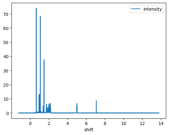
NMR.plot(x='shift', y='intensity')

<AxesSubplot: xlabel='shift'>

../_images/Unit_10_NMR_application_solution_20_1.png

2.3 - Read in all NMR files#

Now we can read one file, we should write a function that can read them all.

def read_NMR_data(NMR):
    """ Read NMR data. """

    data = pd.read_csv(NMR, sep='\t', names=['shift','intensity','derivative'])
    return data

read_NMR_data('data/NMR_data/10.txt')
    

	shift	intensity	derivative
0	14.202218	-0.064711	0.059473
1	14.201989	-0.066458	0.048571
2	14.201760	-0.056322	0.038129
3	14.201530	-0.040992	0.040142
4	14.201301	-0.034111	0.052170
...	...	...	...
65531	-0.826316	-0.058335	0.063376
65532	-0.826545	-0.066090	0.063032
65533	-0.826775	-0.070918	0.056772
65534	-0.827004	-0.069708	0.051623
65535	-0.827233	-0.069516	0.051118

65536 rows × 3 columns

NMR_data = {}
for ID in summary.index:
    NMR_file = 'data/NMR_data/' + str(ID) + '.txt'
    NMR_data[ID] = read_NMR_data(NMR_file)
    
NMR_data[11]

	shift	intensity	derivative
0	13.808344	-0.063278	0.077326
1	13.808115	-0.059682	0.071795
2	13.807885	-0.054798	0.070505
3	13.807656	-0.052117	0.071388
4	13.807427	-0.050141	0.071391
...	...	...	...
65531	-1.220190	-0.057293	0.056825
65532	-1.220420	-0.056044	0.069937
65533	-1.220649	-0.065017	0.077379
65534	-1.220878	-0.074770	0.075543
65535	-1.221108	-0.079670	0.068632

65536 rows × 3 columns

3. NMR data exploration#

To answer the problem

Do you get more peaks in the ¹H NMR spectrum if you have an odd number of heteroatoms compared with an even number?

we will need to determine the number of peaks in a spectrum.

Questions to ask of the data

To peak search automatically, we need the NMR data to have similar numerical values. Things to check are:

What range of chemical shift do they cover?
What is the maximum intensity?
How noisy is the baseline?

Task 3#

Exploring the data:

Write a function that can quantify the following information:
- Range of chemical shifts
- Maximum intensity
- Level of noise in the spectrum background
Extract and store these values for all NMR data
Plot histograms of each of each parameter, and decide whether any corrections to the data are required
Make any corrections required

3.1/3.2 - Extract key features from each spectrum#

# Calculate shift range
min_shift = NMR_data[1]['shift'].min()
max_shift = NMR_data[1]['shift'].max()
shift_range = max_shift - min_shift

print( f"Spectrum covers {shift_range:.3f} ppm from {min_shift:.3f} to {max_shift:.3f} ppm.")

# Calculate max intensity
max_intensity = NMR_data[1]['intensity'].max()
print( f"Maximum intensity is {max_intensity:.3f}.")

# Calculate baseline
number_of_points = NMR_data[1].shape[0]
baseline_std = NMR_data[1]['intensity'].nsmallest(n = int(number_of_points*0.5)).std()
print( f"Baseline noise is {baseline_std:.3f}.")

Spectrum covers 15.029 ppm from -1.233 to 13.796 ppm.
Maximum intensity is 74.038.
Baseline noise is 0.016.

# Now, we convert the code above into a function that can work for any NMR DataFrame

def summary_statistics(NMR_data, ID):
    """ Return summary statistics for an NMR spectrum. """
    
    # Calculate shift range
    min_shift = NMR_data[ID]['shift'].min()
    max_shift = NMR_data[ID]['shift'].max()
    shift_range = max_shift - min_shift

    # Calculate max intensity
    max_intensity = NMR_data[ID]['intensity'].max()

    # Calculate baseline
    num_points = NMR_data[ID].shape[0]
    baseline_std = NMR_data[ID]['intensity'].nsmallest(n = int(num_points*0.5)).std()
    
    return shift_range, max_intensity, baseline_std

for ID in summary.index:
    stats = summary_statistics(NMR_data, ID)
    summary.loc[ID, ['shift_range', 'max_intensity', 'baseline_std']] = stats
    
summary.head()

	heteroatom_count	shift_range	max_intensity	baseline_std
Molecule_ID
1	0	15.029452	74.038383	0.016211
2	2	15.029452	39.278263	0.023142
3	1	15.029451	95.329765	0.018059
4	1	15.029451	22.837284	0.010094
5	2	15.029451	265.857788	0.013083

summary.describe()

	heteroatom_count	shift_range	max_intensity	baseline_std
count	58.000000	58.000000	58.000000	58.000000
mean	2.086207	15.126457	505.006272	0.029138
std	1.013669	0.738770	2500.020776	0.092283
min	0.000000	15.029451	17.880037	0.005242
25%	1.250000	15.029451	57.246149	0.013050
50%	2.000000	15.029452	134.940987	0.016268
75%	3.000000	15.029452	269.394150	0.020450
max	6.000000	20.655757	19181.949219	0.718201

3.3 - Plot histograms across all NMR data#

fig = plt.figure()
ax = fig.add_subplot()
summary['shift_range'].plot(kind='hist', bins=50, ax=ax, label='ppm range')
ax.set_xlabel('Chemical shift range')

Text(0.5, 0, 'Chemical shift range')

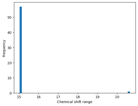
../_images/Unit_10_NMR_application_solution_32_1.png

fig = plt.figure()
ax = fig.add_subplot()
summary['max_intensity'].plot(kind='hist', bins=50, ax=ax, label='Maximum intensity')
ax.set_xlabel('Maximum intensity')

Text(0.5, 0, 'Maximum intensity')

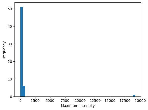
../_images/Unit_10_NMR_application_solution_33_1.png

fig = plt.figure()
ax = fig.add_subplot()
summary['baseline_std'].plot(kind='hist', bins=50, ax=ax, label='Baseline sigma')
ax.set_xlabel('Baseline standard deviation')

Text(0.5, 0, 'Baseline standard deviation')

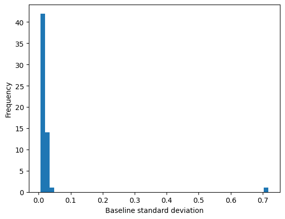
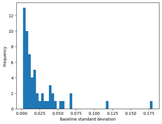
../_images/Unit_10_NMR_application_solution_34_1.png

3.4 - Apply corrections to standardise the data#

For peak searching to work effectively, we need to standardise our data. The simplest change would be to normalise the intensity values so that, e.g. the maximum is 100.

for ID in summary.index:
    NMR_data[ID]['intensity'] = NMR_data[ID]['intensity'] / NMR_data[ID]['intensity'].max() * 100

for ID in summary.index:
    stats = summary_statistics(NMR_data, ID)
    summary.loc[ID, ['shift_range', 'max_int', 'baseline_std']] = stats

fig = plt.figure()
ax = fig.add_subplot()
summary['baseline_std'].plot(kind='hist', bins=50, ax=ax, label='Baseline sigma')
ax.set_xlabel('Baseline standard deviation')

Text(0.5, 0, 'Baseline standard deviation')

../_images/Unit_10_NMR_application_solution_38_1.png

NMR peak hunting#

A number of different peak finding algorithms exist, but here we will focus on scipy.signal.find_peaks that you saw in unit 7. Use this to determine the number of peaks in each NMR spectrum, and store these values for plotting. We can optimise the peak finding using the prominence parameter (in this case; other problems might need different parameters).

Task 4#

Finding Peaks:

Write a function capable of extracting peaks from any of the NMR spectra
Test how the peak-fitting parameters affect the number of peaks determined

Hint: “prominence” is particularly useful for these peak shapes
Optimise these parameter(s) to determine the number of peaks in each spectrum

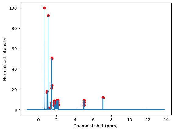
4.1 - Function to extract peaks#

ID = 1
peaks, peak_info = find_peaks(NMR_data[ID]['intensity'],
                              prominence = 1,
                             )


fig = plt.figure()
ax = fig.add_subplot()

ax.plot(NMR_data[ID]['shift'], NMR_data[ID]['intensity'])
ax.scatter(NMR_data[ID]['shift'][peaks],
           NMR_data[ID]['intensity'][peaks],
           color='r'
          )

ax.set_xlabel('Chemical shift (ppm)')
ax.set_ylabel('Normalised intensity')

#ax.set_xlim(7.3,8)
#ax.set_ylim(0,20)

Text(0, 0.5, 'Normalised intensity')

../_images/Unit_10_NMR_application_solution_42_1.png

def count_peaks(NMR_data, ID, prominence):
    """ Return the number of peaks in an NMR spectrum. """
    
    peaks, peak_info = find_peaks(NMR_data[ID]['intensity'],
                                  prominence = prominence,
                                  )
    
    return len(peaks)

4.2 - Optimising the prominence parameter#

To find peaks automatically we need to choose a prominence value. Let’s systematically test a few different ones and see what the effect is on number of peaks. There are many ways to tackle this, but here we’ll use the power of pandas to plot multiple curves quickly (and neatly)!

prominence_range = np.arange(0.1, 5, 0.2)


# Make an empty DataFrame with 'prominence value' as the row index and 'ID' as the columns
prom_testing = pd.DataFrame(index=prominence_range, columns=summary.index)

for prom in prom_testing.index:
    for ID in prom_testing.columns:
        prom_testing.loc[prom, ID] = count_peaks(NMR_data, ID, prom)

ax = prom_testing.plot(figsize=(10,8), colormap='viridis')
ax.set_xlabel('Prominence')
ax.set_ylabel('Number of detected peaks')
ax.legend(ncol=5)

<matplotlib.legend.Legend at 0x7fa3f3756610>

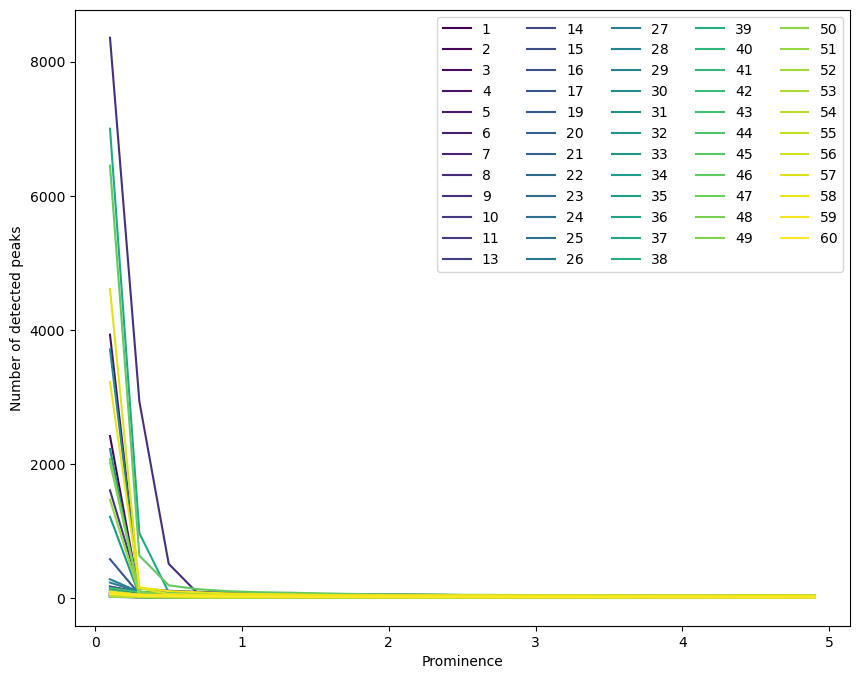
../_images/Unit_10_NMR_application_solution_46_1.png

Click here to see some discussion on the prominence parameter.

A prominence above ~1 seems to give a fairly constant number of peaks, but anything below this gives a number of peaks strongly dependent on this parameter.

We will choose prominence = 1 to avoid biasing the number of peaks in one spectrum over another. It is possible that we are missing some “real” peaks, but we are unlikely to do better in one spectrum than another.

4.3 - Optimise the parameters and extract peak count#

# Calculate number of peaks using optimum prominence value
for ID in summary.index:
    summary.loc[ID,'num_peaks'] = count_peaks(NMR_data, ID, prominence=1)

5. Analysing the results#

Now we have computed the number of peaks, we can this for each spectrum in order to answer the original question.

Task 5#

Plotting:

Plot graphs to determine whether the number of heteroatoms influences the number of NMR peaks.

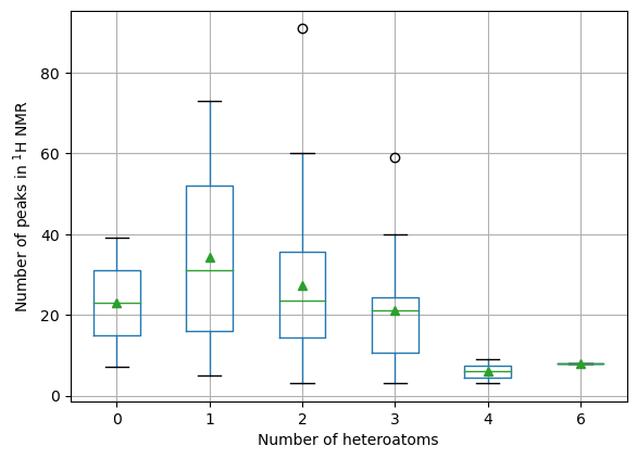
ax = summary.boxplot(column = 'num_peaks', by='heteroatom_count', showmeans=True)
ax.set_xlabel('Number of heteroatoms')
ax.set_ylabel('Number of peaks in $^1$H NMR')

# We need these lines to remove the additional "title" text
# (try commenting them to see what happens)
ax.set_title('')
ax.get_figure().suptitle('')

Text(0.5, 0.98, '')

../_images/Unit_10_NMR_application_solution_52_1.png

summary['even_heteroatoms'] = (summary['heteroatom_count'] % 2) == 0

ax = summary.boxplot(column = 'num_peaks', by='even_heteroatoms', showmeans=True)
ax.set_xlabel('Number of heteroatoms')
ax.set_ylabel('Number of peaks in $^1$H NMR')

# We need these lines to remove the additional "title" text
# (try commenting them to see what happens)
ax.set_title('')
ax.get_figure().suptitle('')

Text(0.5, 0.98, '')

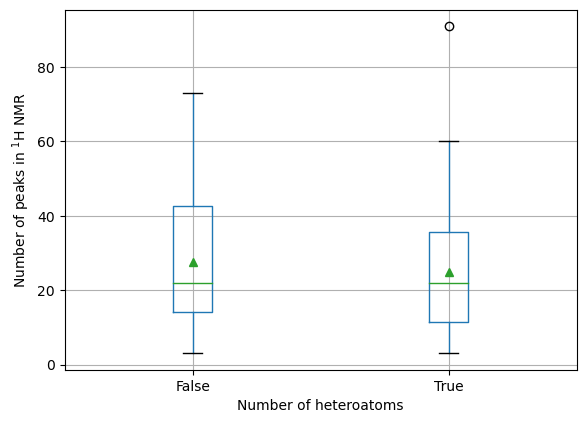
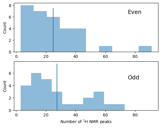
../_images/Unit_10_NMR_application_solution_54_1.png

fig = plt.figure()
ax1 = fig.add_subplot(211)
ax2 = fig.add_subplot(212, sharex=ax1)
ax1.hist(summary[summary['even_heteroatoms']]['num_peaks'], alpha=0.5)
ax2.hist(summary[~summary['even_heteroatoms']]['num_peaks'], alpha=0.5)

ax2.set_xlabel('Number of $^1$H NMR peaks')
ax1.set_ylabel('Count')
ax2.set_ylabel('Count')

ax1.text(75,6.5, 'Even', fontsize=14)
ax2.text(75,5, 'Odd', fontsize=14)

ax1.vlines(summary[summary['even_heteroatoms']]['num_peaks'].mean(), 0, 7.5)
ax2.vlines(summary[~summary['even_heteroatoms']]['num_peaks'].mean(), 0, 7.5)

<matplotlib.collections.LineCollection at 0x7fa3f38bdf40>

../_images/Unit_10_NMR_application_solution_55_1.png

Conclusions#

Key points:

The number of ¹H NMR peaks appears to decrease with increasing numbers of heteratoms
- This may just be due to a smaller number of compounds in this range
Molecules with one heteroatom show the highest number of NMR peaks on average
Comparing odd with even numbers of heteratoms, there is little evidence from these data of any difference
- Further work would be to apply statistical testing on these distributions, ideally using a greater number of measurements.

Tasks to complete after this session#

Read through the notebook with answers, and check that you have understood the steps
Find and read the documentation for any Python commands you are less familiar with
Think about other ways to solve the problem, and try to implement/compare them
Extend your analysis to explore other peak searching approaches (or parameters)
Use statistical methods you have learned to quantify any correlations we have observed

Data-Driven Chemistry

Unit 10: Solutions to Analysing NMR Data from Start to Finish

Contents