Unit 03: Loops, Pandas and Simple Plotting II#

Author: Dr Claire Hobday

Email: claire.hobday@ed.ac.uk

Learning objectives:#

By the end of this unit, you should be able to

use in-built functionality in Python
import modules and libraries
use the math module to do some simple scientific computing tasks
develop more pandas skills to deal with large volumes of data
use logical operations to filter data
understand and use the different types of loops to do repetitive tasks including:
- for
- if
- else/elif
- while
- break
combine these tools to analyse data in a large file containing information about the periodic table
use tools from Python to understand trends in the periodic table

Some of the material was adapted from Python4Science, as well as Software Carpentries.

Table of Contents#

Boolean Indexing
1.1. Tasks 1
Using Pandas DataFrames with loops to analyse data
Plotting with Pandas
3.1 Tasks 2

Jupyter Cheat Sheet

To run the currently highlighted cell and move focus to the next cell, hold ⇧ Shift and press ⏎ Enter;
To run the currently highlighted cell and keep focus in the same cell, hold ⇧ Ctrl and press ⏎ Enter;
To get help for a specific function, place the cursor within the function’s brackets, hold ⇧ Shift, and press ⇥ Tab;

Links to documentation#

You can find useful information about using math and pandas at

Import libraries#

Run the cell below to import all the required libraries

import numpy as np
import matplotlib.pyplot as plt
import pandas as pd

1. Boolean idexing #

Related to if, elif and else conditions are Booleans.

George Boole was a 19th century self-taught English mathematician, philosopher and logician. He is known for Boolean algerbra, that is based on variables being True or False, denoted as 1 and 0 respectively.

The operations in Boolean algebra are and denoted as \(\wedge\), or denoted as \(\vee\) , and not denoted as \(\neg\).

Venn diagram

In fact, in using if we have already asked python to do a Boolean operation. If our answer to our if statement is true, we continue with our conditional loop. The return of the Boolean variable true or false is what determines the fate of our if loop.

Bitwise Operators#

In python there are many ways to do the same Boolean operations, we are going to use Bitwise operators which compare binary

Operator	Name	Description
`&`	AND	Sets each bit to 1 if both bits are 1
\|	OR	Sets each bit to 1 if one of two bits is 1
`^`	XOR	Sets each bit to 1 if only one of two bits is 1
`~`	NOT	Inverts all the bits
`<<`	Zero fill left shift	Shift left by pushing zeros in from the right and let the leftmost bits fall off
`>>`	Signed right shift	Shift right by pushing copies of the leftmost bit in from the left, and let the rightmost bits fall off

Boolean Tests #

Boolean tests on an array produce an array of booleans:

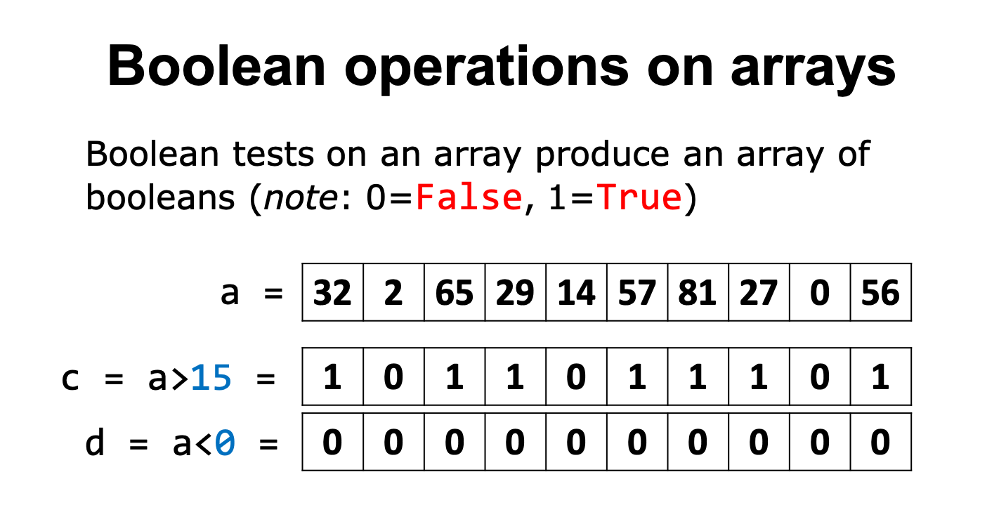
What we can see here is for each value in this series, what the Boolean outcome would be for two tests.

# Declare a series dataframe (just 1D dataframe, like one column of an excel sheet)
a = pd.Series([32, 2, 65, 29, 7, 14, 57, 81, 27, 0, 56])

# Take a look at the format of the series
# "\n" means new-line, so the variable gets printed on the line below followed by an empty line 
print(f"Series a \n {a} \n") 

# Declare tests
c = a[a > 15]
d = a[a < 0]

print (f"condition c = a>15 \n {c} \n")
print (f"condition d = a<0 \n {d} \n")

Both tests c and d are satisfied one after the other. What if we want to satisfy both tests at the same time?

# AND logic
print(c & d)

Here, you can see the output is False, and shows you all the indices where they are False.

Now if we try or :

# OR logic
print(c | d)

Boolean Indexing in Series #

We can also use an array of booleans to index another array, i.e. only elements coresponding to True are extracted from the indexed array.

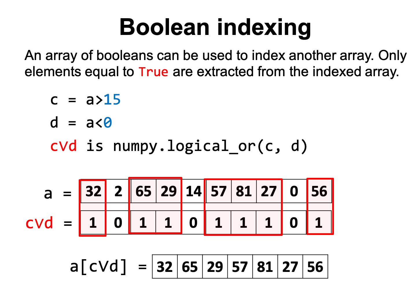
c = a > 15
d = a < 0
a_cVd = a[c | d]
print(a_cVd)

Boolean Indexing in DataFrames#

Using these same logical principles, we can index whole dataframes to recover just the data we need. Let’s take a look at the dataframe below:

# Dictionary of lists
dict = {"name":["Toni", "James", "Claire", "Valentina"],
        "degree": ["Chemistry", "Medicinal and Biological Chemistry", "Chemical Physics", "Chemical Physics"],
        "score":[90, 77, 61, 98]}
 
# creating a dataframe from a dictionary
df = pd.DataFrame(dict)

print(df)

Now let’s use the comparison operator to filter just those who do MBC.

# Using a comparison operator for filtering of data
    
criterion = df["degree"] == "Medicinal and Biological Chemistry"
print(criterion)

# Apply the indexing to our dataframe to return only those that fit our criteria
print(df[criterion])

# Apply the indexing to our dataframe to return only those that DO NOT fit our criteria
print(df[~criterion])

Tasks 1 #

Task 1.1: Mass spectrometry

Using the mass spectometry data in the file ms.txt, find m/z values in the region between m/z 6400 and 6600.

# FIXME
# Read the file ms.txt into the dataframe, and make sure to give the data column names
ms_data = pd.read_csv(filepath_or_buffer=____, sep=___, header=____, names = [_____])

# Criteria for slicing data
# FIXME
print(output)

Click here to see solution to Task 1.1

ms_data = pd.read_csv(filepath_or_buffer="files/ms.txt", sep="\t", header=None, names=["m/z", "intensity"])

# Criteria for slicing data
criterion_1 = ms_data["m/z"] > 6400
criterion_2 = ms_data["m/z"]< 6600
output = ms_data[criterion_1 & criterion_2]
print(output)

Explanation: we need to know the path to the file, look at the file to work out how the columns of data are separated, does the data have headers? What should the column names be?

Task 1.2 : Assess at what m/z value there is a peak between 6400 and 6600.

# FIXME

Click here to see solution to Task 1.2

intensity = output["intensity"]
m_z = output["m/z"]
max_value = intensity.max()
max_index = intensity.idxmax()

print("peak", max_value, "at m/z", m_z[max_index])

2. Using Pandas DataFrames with loops to analyse data #

We are now going to play around with the dataframe we looked at earlier containing information about the periodic table and pull out some more information from this.

ptable = pd.read_csv("files/ptable.csv")

# The entries in the df are ordered 0 to 117 for each element. 
# 0 is hydrogen.
print(ptable.loc[0, :]) 

We can see that there are some variables which return NaN (which stands for “Not a Number”), we can remove or fill these values easily in pandas.

# drop all values
ptable.dropna() 
# or fill with zeros 
ptable.fillna(0)

We are going to add a new column to our dataframe, which will calculate the mass number from the number of neutron and protons which we already have in two columns. This is just done as a simple addition of the two columns.

# add new column to the dataframe
ptable["Calculated_mass_number"] = ptable["NumberofNeutrons"] + ptable["NumberofProtons"]

Calculate the difference between our calculated value Calculated_mass_number and the value given in the array originally AtomicMass.
Think about why the values would be different.

ptable["Difference_in_mass"] = ptable["Calculated_mass_number"] - ptable["AtomicMass"]
for i in range(len(ptable)):
    name = ptable.iloc[i,1]
    difference = ptable.iloc[i, -1]
    print(f"Difference in mass for {name}, {difference}")

Now let’s use some Boolean logic on the periodic table data. Below we will look for all elements that exist as solid as standard temperature and pressure.

solids = ptable[ptable["Phase"] =="solid"]
solids

Task 1.3 : Set boolean tests to check what elements are liquid at 297 K, and extract the names of those elements.

# What columns from the dataframe will we need?

# FIXME

# Set Boolean tests to check what is liquid at 297 K (room T)

# FIXME

# Run the test and print names of elements that are liquid at room temperature

# FIXME

Click here to see the full solution to Task 1.3

    
# What columns from the dataframe will we need?    
element = ptable["Element"]
melting = ptable["MeltingPoint"]
boiling = ptable["BoilingPoint"]
    
# Boolean to check what is liquid at 297 K (room T)
    
temperature_1 = melting < 297
temperature_2 = boiling > 297

criteria = temperature_1 & temperature_2
print(element[criteria])

3. Plotting with Pandas #

Plotting can be done in many ways within python. At first we will just use plotting straight from pandas. It uses a popular library matplotlib in the background. As we progress to later sessions we will use this directly, but for now we will just stick to pandas plotting.

We can use the pandas dataframe to easily plot columns with matplotlib.

The easiest thing we could do, would be to plot all variables against our index

with:

ptable.plot()

However, we can see that this is not very informative, and we must use our knowledge that we have learned in the previous session and earlier in this session to plot the data more sensibly.
We can access what columns we can plot against each other with this command:

ptable.columns

Now, let’s take two variables from the column headers and plot them against each other.
Let’s see if we can see trends in the periods of the periodic table.

ptable.plot.scatter(x = "AtomicNumber", y = "AtomicRadius")

We can clearly see the trends of each period in the periodic table.

Now lets try another type of plot which isn’t scatter. We can use a pie chart to show how many elements were discovered in each location.

Pandas has a handy values_counts() function that we can use on our column of this data.

counting = ptable.discovery_location.value_counts()
print(counting)

# Then we can plot these data as a piechart

counting.plot.pie(figsize=(10,10))

We can also loop over our columns in ptable and plot them as a function of “Element”.

for i in ptable.columns[4:9]:
    print(i)
    fig = plt.figure(figsize=(15,10))
    plt.plot(ptable["Element"], ptable[i])
    plt.xticks(rotation=90)
    plt.show()
    
# Note how we rotate the xticks 90 degrees to see the name on its side!

Tasks 2 #

Task 2.1: Selecting individual values in a dataframe

Using the ptable dataframe, write an expression to find and print the boiling point of argon.

# FIXME

Click here to see solution to Task 2.1

Like most things in python, this can be approached in a few ways, e.g. we know that Argon is the 18th element in the periodic table, therefore it is going to be index 17 in our dataframe (python counts from zero)

print(ptable.loc[17, "BoilingPoint"])

Another way to search for this would be to do some Boolean indexing.

criteria_ar = ptable["Element"] == "Argon"
print(criteria_ar) 
print(ptable[criteria_ar]["BoilingPoint"])
  

Task 2.2: Slicing dataframes

Have a look at these two ways of slicing, what is different about them?

print(ptable.iloc[4:6, 1:3])

print(ptable.loc["4":"6", "AtomicNumber":"Symbol"])

Click here to see solution to Task 2.2

Notice how the second statement produces additional columns and many additional row compared to the first statement.

What conclusion can we draw? We see that a numerical slice, (first example) omits the final index (i.e. 6) in the range provided, while a named slice, "AtomicNumber":"Symbol", includes the final element “Symbol”.

A funny quirk of not naming our index is that all rows between 40 and 60 are printed with the second method.

Task 2.3: Use a loop to identify all symbols with 1 letter

Using the symbol column in the dataframe ptable use a loop to identify and count all the elements which have a one letter symbol.

# FIXME

Click here to see solution to Task 2.3

one_etter= []
for x in ptable["Symbol"]:
    if len(x) < 2:
        one_letter.append(x)
len(one_letter)

Data-Driven Chemistry

Unit 03: Loops, Pandas and Simple Plotting II

Contents