Unit 08: Applications to Chemistry – Mass Spectrometry and Radioactive Decay#

Authors:

Dr Valentina Erastova
Dr Matteo Degiacomi
Hannah Pollak

Learning Objectives#

This is the first of two Units focussing on applying the learned material for chemistry-related problems. In this Unit you will:

look at the real mass spectrometry data for some interesting molecules, visualise the structures, plot the data and find the peaks.
learn about carbon isotopes, their stability and radioactive decay, and how we can use it to calculate the age of a given sample.
make a Quiz, that could even be helpful for you to learn periodic table.

Table of Contents#

Real Mass Spectrometry data of a fun molecule
1.1 Visualising Molecular Structure
1.2 TASK 1 & 2 - Finding Peaks
Radioactive Decay
2.1 Theoretical background - radiocarbon
2.2 Exponential decay - Let’s run a simulation
2.3 TASK 3 - Finding the half-life from the decay data collection
Write a Chemistry Quiz
3.1 What makes a good Quiz?
3.2 Structure of a Quiz
3.3 TASK 4 & 5 - Write (and play) a Quiz

Application 1: Real Mass Spectrometry data of a fun molecule#

Mass Spectrometry (MS) is an experimental technique enabling the measurement of the mass-to-charge (m/z) of a molecule. In a mass spectrometer, molecules can also be fragmented: as such, the mass-to-charge of resulting fragments can also be simultaneously detected. A typical mass spectrum is reported in a dataset with two columns: the first is a regularly spaced range of m/z values, while the second is the detected intensity associated with each m/z value. In this first application, we will work with MS data of some fun molecules!

By running the cell below, a random molecule will be selected. The following information will be returned:

a name of one of the molecules (saved in the variable m)
a link to the The Molecule of the Month website associated to your molecule (saved in the variable w).

Printed on screen, you will find the path to text files containing the molecular structure and MS data.

The MS data for all the compounds is taken from MassBank. ACCESSION, RECORD_TITLE, DATE and AUTHORS are given in the comment section (lines starting with #) of the data/MS_*Molecule*.txt file.
The molecular structures are obtained from MolView.

The Molecule of the Month website, created by Prof Paul May from Bristol University, holds information on many of the interesting molecules that we meet in our lives. For more information, see: P.W. May, S.A. Cotton, K. Harrison, H.S. Rzepa, The ‘Molecule of the Month’ website – an extraordinary chemistry educational resource online for over 20 years”, Molecules 22 (2017) 549-559

import molecule_getter as mg
m, w = mg.get_molecule()

1.1 Visualising Molecular Structure#

The molecule selected for us has its name saved in the variable m. The molecule itself (as a .mol file), is available in the data directory of this unit. Let’s store in the variable molecule the path to .mol file.

molecule = f'./data/{m}.mol'

Let’s start by visualising our molecule. For this we can use the nglview Python package (see its documentation here).

import nglview as nv

molec = nv.show_file(molecule)
molec

molec.add_surface(opacity=0.2) # add a surface representation

molec.color_by('atomindex') # colour by index

If we want to change the representation completely, we need to first clear the previous representations, then add the new one.

molec.clear_representations()
molec.add_hyperball(color='white')
molec.add_hyperball(selection='atom _O', color='red')

1.2 Finding peaks on MS data#

TASK 1 - Finding peaks on your MassSpec

Load the data from the mass spectrum in the .txt file named above
Label with a cross the highest peak in the txt file, and find its corresponding m/z
add labels and legends to your plot, and save it
What is the difference between intensity and relative intensity? Calculate the relative intensity and produce a correctly labelled plot.
Using scipy.signal.find_peaks, find all peaks in the dataset, and mark them with a cross.

HINTS:

Do you remember what molecule it was?

The variable defining your molecule is m, you can print it in the terminal:

print(f'Your molecule is {m}, and the datafile is data/MS_{m}.txt')

Do you know how your datafile looks like? What are the comments and the delimeters?

Before loading the mass spectrum data into our notebook we should take a closer look at what the datafile looks like.

!head -24 ./data/filename.txt

You should find that the file is has comments on the lines starting with ‘#’; the data is in 3 columns: m/z, intensity, relative intensity, separated by the white spaces.

Do you need a help to load datafiles?

See Session 5 extra notebook Pandas vs Numpy

Do you need a reminder on plotting?

See Session 5 extra notebook Plotting

To annotate your plot:

you can use function plt.annotate ('text', xy=(x,y) ) more information here in the case of this example the text will be m/z= VALUE and can be expressed like this: mz = %s'%maxval[0] the position is slightly offset from the peak itself (maxval[0]+10, maxval[1]-50)

To find peaks:

package you have already seen scipy.signal.find_peaks manual here

we will see that the input should look like this:

peaks, _ = find_peaks(x) 

where _ is used for an array that you will not use (see later details for this); where x is our signal the other parameters are non-compulsory, but necessary for a good search.

# Do you remember what is your molecule?

# Your Solution

SOLUTION on an example of Caffeine using numpy only:

import numpy as np

import matplotlib.pyplot as plt
plt.rc('font', family='serif', size=12)

from scipy.signal import find_peaks

#load data
data = np.loadtxt("./data/MS_Caffeine.txt", comments='#')

#assign columns to variable names
mz = data[:, 0]
intens = data[:, 1]
relintens = data[:, 2]

#find max in intensity and it's position
maxpos = np.argmax(intens)
maxval = data[maxpos, :]
print('Max m/z is', maxval[0])

#find peaks
peaks, _ = find_peaks(relintens)
print('found', len(peaks), 'peaks')

#make a figure
plt.figure(figsize=(10, 6))

plt.subplot(1, 2, 1, title="Caffeine MS - single peak")

#add data to the plot
plt.plot(mz, intens, '-', c='c', label='data')
plt.plot(maxval[0], maxval[1], 'X', c='r', label='peak')

#adding an value next to the peak
x = maxval[0] + 10  #shift x axis to the right by 10
y = maxval[1] - 50  #shift y axis down by 50
plt.annotate('m/z=%s' % maxval[0], xy=(x, y))

#plot legend with a location and label axis
plt.legend(loc='upper left')
plt.xlabel("m/z")
plt.ylabel("intensity")

#next plot
plt.subplot(1, 2, 2, title=f'Caffeine MS - top {len(peaks)} peaks')
plt.plot(mz, relintens, '-', c='c', label='data')
plt.plot(data[peaks, 0], data[peaks, 2], 'X', c='r', label='peaks')

#label and adjust plot
plt.legend()
plt.xlabel("m/z")
plt.ylabel("relative intensity")
plt.subplots_adjust(wspace=0.3)

#save figure ans show the plot
plt.savefig("MS_Caffeine_MZ.png")
plt.show()

SOLUTION on an example of Caffeine using pandas:

import pandas as pd

import matplotlib.pyplot as plt
plt.rc('font', family='serif', size=12)

from scipy.signal import find_peaks

#load data and assign column labels
data = pd.read_csv("./data/MS_Caffeine.txt",
                   sep='\s+',
                   comment='#',
                   names=['mz', 'I', 'relI'])

#select 'm/z' as the index column
data.set_index('mz', inplace=True)

# one option for finding maximum intensity and mz at that position
# use idxmax to select index where column 'I' is max
# use max for finding maximum in 'I' column
max_val = data['I'].idxmax()
max_pos = data['I'].max()
print(f'm/z of max I is {max_val}\n' f'max I is {max_pos}\n')

# find peaks in 'relI' column
peaks, _ = find_peaks(data['relI'])
print('found', len(peaks), 'peaks')

#make a figure
plt.figure(figsize=(10, 6))

plt.subplot(1, 2, 1, title="Caffeine MS - single peak")

#add data to the plot
plt.plot(data.index, data['I'], '-', c='c', label='data')
plt.plot(max_val, max_pos, 'X', c='r', label='peak')

#adding an value next to the peak
x = max_val + 10  #shift x axis to the right by 10
y = max_pos - 50  #shift y axis down by 50
plt.annotate(f'm/z={max_val}', xy=(x, y))

#plot legend with a location and label axis
plt.legend(loc='upper left')
plt.xlabel("m/z")
plt.ylabel("intensity")

#next plot
plt.subplot(1, 2, 2, title=f'Caffeine MS - top {len(peaks)} peaks')
plt.plot(data.index, data['relI'], '-', c='c', label='data')
plt.plot(data.iloc[peaks, 1].index,
         data.iloc[peaks, 1],
         'X',
         c='r',
         label='peaks')

#label and adjust plot
plt.legend()
plt.xlabel("m/z")
plt.ylabel("relative intensity")
plt.subplots_adjust(wspace=0.3)

#save figure ans show the plot
plt.savefig("MS_Caffeine_MZ.png")
plt.show()

TASK 2 - Optimise the Search

Optimise the search for peaks:

scipy.signal.find_peaks(x, height=None, threshold=None, distance=None, prominence=None, width=None, wlen=None, rel_height=0.5, plateau_size=None)

the output will then also give a dictionary of various properties, according to the parameters passed.

Try 4 searches, setting the various height, threshold, distance, prominance and see how it affects the peak search, by plotting these next to each otheras 2x2 grid of subplots

# Your Solution

SOLUTION on an example of Caffeine:

import numpy as np

from scipy.signal import find_peaks

data = np.loadtxt("./data/MS_Caffeine.txt", comments='#')

#lets use normalised data
intens = data[:, 2]

#define parameters the test
h = 20
p = 100
w = 1
t = 10

peaks1, properties1 = find_peaks(intens, height=h)
print('found', len(peaks1), 'peaks for height=', h)

peaks2, properties2 = find_peaks(intens, prominence=p)
print('found', len(peaks2), 'peaks for prominence=', p)

peaks3, properties3 = find_peaks(intens, height=h, width=w)
print('found', len(peaks3), 'peaks for hight = %s and width=%s' % (h, w))

peaks4, properties4 = find_peaks(intens, threshold=t)
print('found', len(peaks4), 'peaks for threshold=', t)

#plot it
plt.figure(figsize=(10, 8))

plt.subplot(2, 2, 1)
plt.plot(data[peaks1, 0], data[peaks1, 2], "xr")
plt.plot(data[:, 0], data[:, 2], 'c')
plt.legend(['height'])

plt.subplot(2, 2, 2)
plt.plot(data[peaks2, 0], data[peaks2, 2], "xb")
plt.plot(data[:, 0], data[:, 2], 'c')
plt.legend(['prominence'])

plt.subplot(2, 2, 3)
plt.plot(data[peaks3, 0], data[peaks3, 2], "xm")
plt.plot(data[:, 0], data[:, 2], 'c')
plt.legend(['hight & width'])

plt.subplot(2, 2, 4)
plt.plot(data[peaks4, 0], data[peaks4, 2], "xk")
plt.plot(data[:, 0], data[:, 2], 'c')
plt.legend(['threshold'])

plt.savefig("MS_Caffeine_Peaks_compare.png")

plt.show()

Feeling like you want to analyse and plot more data?

There are a few more data files for you, providing data on compounds typically used as calibrants in MS.

MS_FC43pos.txt Perfluorotributylamine (FC43), here as a positive ion
MS_FC43neg.txt FC43 as a negative ion
MS_PFK.txt Perfluorokerosene (PFK)
MS_FC70pos.txt Perfluorotripentylamine (FC70) pssitive
MS_FC70neg.txt FC70 negative ion
MS_FAB.txt
MS_CsI.txt

SOLUTION example:

#load data
data1 = np.loadtxt("./data/MS_FC43pos.txt", comments='#')
data2 = np.loadtxt("./data/MS_FC43neg.txt", comments='#')

#find max and min
maxpos1 = np.argmax(data1[:, 1])
maxval1 = data1[maxpos1, :]
maxpos2 = np.argmax(data2[:, 1])
maxval2 = data2[maxpos2, :]

#make a figure
plt.figure()

#make subplot, name the figure
plt.subplot(1, 1, 1, title="Perfluorotributylamine")

#add data to the plot
plt.plot(data1[:, 0], data1[:, 1], '.-', c='c', label='Positive Ion')
plt.plot(data2[:, 0], data2[:, 1], '.-', c='b', label='Negative Ion')
plt.plot(maxval1[0], maxval1[1], 'X', c='r', label='peaks')
plt.plot(maxval2[0], maxval2[1], 'X', c='r')

#labe  axis
plt.xlabel("m/z")
plt.ylabel("Rel. Abundance")

#plot legend with a location
#'upper/lower left/right/center' or 'center left/right'
plt.legend(loc='upper right')

#save figure
plt.savefig("MS_FC43.png")

plt.show()

Application 2: Radioactive Decay#

1.2 Theory #

Radiocarbon#

Isotopes of an element share the same number of protons but have different numbers of neutrons. Each element has numerous isotopes, but only a few will be stable enough to be found naturally. For example, carbon has:

two stable isotopes:
- 98+% of total carbon is ¹²C, and
- ~1% is ¹³C (¹³C allows us to do NMR!)
one radioactive (i.e. capable of a decay into another element) ¹⁴C, formed cosmogenically in small amounts.
further 12 isotopes are known, only stable on the sub-second timescales they have been produced artificially.

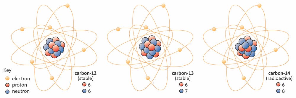
Since Carbon-14 has one too many neutrons, it will undergo a $\beta^-$ decay into ¹⁴N, where a neutron will decay into a proton, emitting an electron ($\beta$-particle) and an anti-neutrino, ν:

₆¹⁴C -> ₇¹⁴N + e^- + ν

The amount of carbon-14 is constantly replenished through the reaction of nitrogen-14 in the atmosphere under exposure to the cosmic ray action:

n + ₇¹⁴N -> ₆¹⁴C + p⁺

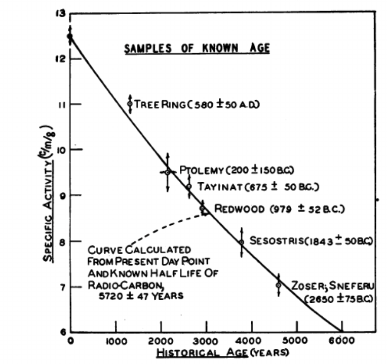
Therefore, ¹⁴C is a cosmogenic nuclide. However, open-air nuclear testing (between 1955 and 1980s) have also increased the amount of ¹⁴C in the environment. This Carbon-14, reacts with oxygen, forming CO₂ and gets incorporated (photosynthesis, mixing, C-exchange) into various living species and natural materials. Decaying slowly with a halflife of 5730 years, it becomes ideal for dating materials up to 10 000 BC (Mesolithic age, when humans have still been mainly hunter/gatherers).

The method of radiocarbon dating was proposed by Willard Libby in 1949. Here is the figure from the original paper explaining the ages of various materials - J. R. Arnold & W. F. Libby, “Age Determinations by Radiocarbon Content: Checks with Samples of Known Age,” Science 110(2869), 678–680, 1949.

Want to learn more?

The Shroud of Turin is a linen cloth, claimed to be the negative image of Jesus of Nazareth, as the cloth wrapped the body after crucifixion. In 1988, radiocarbon dating established that the shroud was from the Middle Ages, between the years 1260 and 1390. P. E. Damon et al., Radiocarbon Dating of the Shroud of Turin, Nature 337(6208), 611–615, 1989.
The Bakhshali Manuscript contains the earliest known Indian use of a zero symbol. There has been some debate on the age of this manuscript.
J. Van der Plicht et al.Recent Developments in Calibration for Archaeological and Environmental Samples, Radiocarbon, 62(4), 1095-1117, 2020.

Radioactive Decay#

The decay itself is exponential - the number of particles, $N$, at a given moment in time, $t$, can be calculated as:

$ N=N_0 e^{-\lambda t}$ ,

where $\lambda$ is the decay constant, $N_0$ is the number of particles at the start, i.e. at $t=0$.

The halflife, $\tau$, of a material is the time it takes for the half of radioactive particles to decay:

$\tau = \frac{\ln(2)}{\lambda}$ .

Let’s see this in action with a simulation below.

2.2 Simulating Radioactive Decay#

Adapted from Wired, written by Rhett Allain.

A material made of element X is composed from stable blue particles and radioactive red particles, which decay into a new element Y, stable cyan particles.

The total amount of particles forming material is 500 element X, out of which 34.4% are radioactive.

The decay rate for the X –> Y is 1/3, i.e a particle has 33.3(3)% chance to decay over a given unit of time.

Below, we calculate what happens over the 1000 time units, and we will run the calculation with a step of 5 time units.

There will be a large print out of the code, change the cell view by:

Cell tab -> All Outputs -> Toggle Scrolling

You likely need to install vpython installed. For this, please run the cell below.

!pip install vpython

# INPUTS FOR THE DECAY

#N is the total number of atoms
N = 500

#N2 is number of atoms that can decay
N2 = 0.344 * N  #0.344 is 34.4%. You could try changing this

#instead of steps, I am using t for time. simulation will run untill tmax
t = 0
tmax = 1000

#dt is the time interval. it is set to 5 time units. You could try changing this
dt = 5

#r is the decay rate - the probability that one atom decays at time interval dt
r = 1 / 3 # rate of 1/3, is a decay chance of 33.3%. You could try changing this


########## PROGRAM BELOW ###########

from vpython import *
# This is needed in Jupyter notebook and lab to make programs glowscript programs rerunnable
canvas(title='<b>Decay Simulation</b>', background=color.white, height=400)  

#Build initial system
atoms = []
atoms2 = []

#n and n2 are counters
n = 0
while n <= (N - N2):
    atoms = atoms + [ sphere(pos=vector(3 * (random() - 1), (3 * random() - 1), 0),
               radius=0.05, color=color.blue, opacity=0.3) ]
    n = n + 1

n2 = 0
while n2 <= N2:
    atoms2 = atoms2 + [ sphere(pos=vector(3 * (random() - 1), (3 * random() - 1), 0),
               radius=0.05, color=color.red) ]
    n2 = n2 + 1

print("Total no. of atoms is %s" %(N))
print( "%.2f%% of them are unstable (=red)," %(N2 * 100 / N))
print ("i.e. at the start of simulation, t=0, there are %i unstable atoms \n " % (N2))

#decay is the number of things that have decayed, starts with 0
decay = 0

#this part makes a graph
g1 = graph(title='<b>Decay plot</b>', xtitle='time',
           ytitle='No. of particles per type', width=600, height=400, fast=False)

f1 = gdots(graph=g1, color=color.blue, radius=3) #points on the plot
#f2 = gcurve(graph=g1) # add a line plot
f3 = gdots(graph=g1, color=color.red, radius=3)
#f4 = gcurve(graph=g1) 
f5 = gdots(graph=g1, color=color.cyan, radius=3)
#f6 = gcurve(graph=g1) 

#add initial data to graph
f1.plot(t, N)
f3.plot(t, N2)
f5.plot(t, decay)

#the following is a loop to go through each item for decay
#this runs as long as t is less than tmax
while t < tmax:
    #rate(10) means display ten loops per second
    rate(10)

    #this goes through each atom in the list and decides if it decays
    for i in atoms2:
        #temp is a random number between 0 and 1. temperature can be thought of as a probability
        temp = random()

    #if it decays, do two things:
    if temp < r:
        #1-make the atom change colour
        i.color = color.cyan
        #i.emissive=True
        #i.visible=False
        #2-remove it from the atom list, add to decay list
        atoms2.remove(i)
        decay = decay + 1
    
    #increase time by one time interval step
    t = t + dt
    
    #add a data point to the graph
    f1.plot(t, (len(atoms2) + len(atoms)))
    #f2.plot(t, (len(atoms2) + len(atoms)))
    f3.plot(t, (len(atoms2)))
    #f4.plot(t, (len(atoms2)))
    f5.plot(t, decay)
    #f6.plot(t, decay)

#prints the number of atoms that decayed at the end of the simulation
print(f'{decay} of unstable atoms (=red) have decayed (=cyan) by the t = {f}')
print(f'There are still {len(atoms2)} atoms that can decay')

2.3 Fitting radioactive decay #

Adapted from: Christian Hill, The Second Edition of Learning Scientific Programming with Python, ISBN: 9781108745918, published by Cambridge University Press in Nov 2020.

TASK 3 - Fit ¹⁴C decay datasets to find half-life $\tau$

The dataset data/14C_MC_sim.csv contains a set of individual decay datapoints for carbon-14 over a series of time.

Load the data (is it commented? are comments useful? what are the separators?)
How many sets are there?
Fit the data to obtain $\tau$ and $N_0$
Plot the fit, as well as the average and standard deviation OR the collection of all datasets.

HINTS:

Average individual simulation datapoints along the colums to use for the fitting:

N = Data.mean(axis=1)

You can calculate STD to plot it as an error bar:

plt.errorbar(t, N, err)

Profit from converting and exponential decay into a linear relation:

$ N = N_0 ~ \exp\left(\frac{-t}{\tau}\right) $ => $\ln(N) = \ln(N_0) \frac{-t}{\tau} $

use np.linalg.lstsq function to perform a linear least-squares fit
OR use non-linear least squares fit, i.e. curve_fit to fit to the exponential function directly. Don’t forget to..

from scipy.optimize import curve_fit

# Your Solution

SOLUTION example:

#load libraries and make some pretty settings
import numpy as np
from scipy.optimize import curve_fit
import matplotlib.pyplot as plt
from matplotlib import cm
plt.rc('font', family='Helvetica', size=14)
import cmocean
cm = cmocean.cm.ice

# Load in the data and separate into a time column, tgrid, and columns of
# simulation runs, Nsim. 
arr = np.loadtxt('data/14C_MC_sim.csv', delimiter=',')
tgrid = arr[:, 0]
npts = len(tgrid)
Nsim = arr[:, 1:]
# Average Nsim for each time point.
N = Nsim.mean(axis=1)
Nstd = Nsim.std(axis=1)


# Least-squares fit to log(N) as a function of t: should be a straight line
def decay(t, N0, tau):
    return N0 * np.exp(-t / tau)


# Initial guesses: estimate tau from the noisy data or a linear fit to log(N)
p0 = N[0], 8000
popt, pcov = curve_fit(decay, tgrid, N, p0)
N0, tau = popt

# Report N0 and the half-life
thalf = np.log(2) * tau
print('Fitted parameters: N_0 = %.1f tau = %.1f years' % (N0, thalf))
NFit = N0 * np.exp(-tgrid / tau)

# PLOT
plt.figure(figsize=(12, 8))

# Plot the averaged data and the fit curve
colors = cm(np.linspace(0, 1, arr.shape[1]))
for i in range(arr.shape[1]):
    plt.plot(tgrid, Nsim[:, 1:], '.', alpha=0.2, c=colors[i])

plt.errorbar(tgrid, N, Nstd, fmt='o', c='dimgrey', label='Average + STD')

# Plot the fit
plt.plot(tgrid,
         NFit,
         c='r',
         label=r'Fit with $N_0$ = %.1f, $\tau$ = %.1f yr' % (N0, thalf))
plt.legend()
plt.xlabel('Time, $t$/yr')
plt.ylabel('Remaining 14-C count, $N(t)$')
plt.savefig('decay-fit-nonlinear.png')
plt.show()

Application 3: Write an Interactive Chemistry Quiz Application#

3.1 Components of a Good Quiz Application #

from IPython.display import HTML, IFrame
HTML('<iframe src=https://www.menti.com/alikv3cbwjwt/embed width=700 height=900></iframe>')

HTML('<iframe src=https://www.mentimeter.com/app/presentation/al9q2arbho621ads5j496qsweyx3nirh/embed width=700 height=400></iframe>')

Prerequisites of a good Quiz application:#

What do you want to test? What questions should you ask? How to make them non-ambiguous?
What are the rules of the Quiz? State them clearly.
Make the application user friendly, communicate to the player, interactivity is key.
Make sure the application is bombproof - user will make mistakes, and should be able to restart.
Keep the code organised: use lists/tuples/dictionaries.
Make sure you are not revealing information you test to the player (esp if running from a Jupyter Notebook, where code is displayed) - hide the data you test against into a file.
Check conditions you test with if statements.
Repeat actions with the for/while loops.
Use functions!
Make your code flexible, easy to expand - odds are you will be keen to add new functionality.
Keep testing by playing!

3.2 Making a Quiz #

Let’s create a quiz that will test the player on their knowledge of periodic table of elements - very chemistry Quiz!

Step 1: Ask your Question#

Make sure to suggest the options for the answer:

startgame = input('Are you ready to start the Game? [Y/n]')

Act on the instructions (=answer) received you will need an if statement.

Remain flexible with the answer! While suggested Y the use could have not paid attention and put a small y instead. Nevertheless, any other letter should be assumed as attempt to quit

if startgame.lower()[0] != 'y':
    sys.exit('Quitting...')

# TRY HERE

Step 2: Check the Answer against some Data#

Hide the questions and answers behind the code into a file.

For example, here we can use this a datafile, containing the information on periodic table:

ptable = pd.read_csv('data/ptable.csv')

Ask the question using the datafile. Here, random is a handy function to randomise the questions (like used in the Application 1)

randel = random.randint(0, 117)

element = ptable.iloc[randel]
    
print(f'What is the name of an element {element['symbol']}? ')
answer = input('')

Check the answer against the datafile. Here you will need an if statement.

Don’t forget the feedback! Even if the user is wrong, it would be good to give them the correct answer!

if answer.lower() == element['name'].lower():
    # feedback
    print('Correct!')
    
else:
    # feedback, incl correct answer!
    print(f'Wrong, it is {element['name']} ')

# TRY HERE

Step 3: no quiz is good without a score!#

Add a count for the score and keep track!

# set the counters
score = 0

ptable = pd.read_csv('data/ptable.csv')

randel = random.randint(0, 117)
element = ptable.iloc[randel]
print(f'What is the name of an element {element['symbol']}?')
answer = input('')

# check the answer
if answer.lower() == element['name'].lower():
    print('Correct!')
    #update the score
    score += 1 
    
else:
    print(f'Wrong, it is {element['name']} ')

# Want to try? or edit the code in the cell above

Step 4: Make Sure the Quiz is not infinite and users can exit#

Even the best quiz has to come to an end!

Ask the user how many Questions they want to play, set the counter as a loop.

# Ask how many questions to set, input should be an intiger!
qcount = int(input('How many questions do you want to brave this time?'))

# print out to confirm
print (f'> You have chosen to do {qcount} questions')

#set the counter 
questions = 0

# start the loop over the number of questions player wants to answer
for i in range(0, qcount):
    
    if answer.lower() == element['name'].lower():
        print('Correct!')
        score += 1 
        questions += 1
    
    else:
        print(f'Wrong, it is {element['name']}')   
        questions += 1

Make sure you have given clear instructions for the game.

print ('I will give you an element, and you will write its symbol. ')
print ('Answers are not case sensitive')

Add a functionality of exiting at any time, and getting the score. This can be within the loop, testing the answers:

print ('You can exit any time by typing `quit`')

# check the answer
if answer.lower() == element['name'].lower():
    print('Correct!')
    score += 1 
    questions += 1
    
elif answer.lower() == 'quit':
    print(f'You got {score} out of {questions} questions!')
    #get out of the loop
    break
    
else:
    print('Wrong, it is %s ' %element['name'])

Now, let’s put this all the elements together in a Quiz!

3.3 Write (and play) your Quiz #

Adapted from: replit.com/@IsaacCHITTILAPP

TASK 4 - Write a quiz about periodic table of elements

Use mendeleev package to get data on the element, its name and atomic number,
or load the datafile data/ptable.csv, already containing the columns ‘symbol’, ‘name’, ‘atomic_number’ for all 117 elements.
Make sure the game is interactive:
How many questions would you like to attempt? ...
Print to the screen to confirm you read in the info right:
> You have chosen to do X questions
Create tests for the input by the user. Did they type in an integer where they should have?
Provide instructions and how to get out:
Answers are not case sensitive
type `quit` at any time to stop the game and get your score
Keep playing, bombproofing your code and adding extra features!

# anything you need to import? 
import random
import mendeleev as mv
import pandas as pd
import sys

# gather data - use mendeleev? 
# what information would you want to include/test?
cols = [ 'symbol', 'name', 'atomic_number']
ptable = mv.get_table('elements')[cols]

# or you can load the file data/ptable.csv prepared for you
#pt = pd.read_csv('data/ptable.csv')

# YOUR QUIZ

SOLUTION example:

import random
import mendeleev as mv
import pandas as pd
import sys

cols = [ 'symbol', 'name', 'atomic_number']
ptable = mv.get_table('elements')[cols]


startgame = input('Are you ready to start the Game? [Y/n]')

# test if they answerred Y or y, any other letter quit
if startgame.lower()[0] != 'y':
    sys.exit('Quitting...')

# Give instructions
print('I will give you an element, and you will write its symbol. ')
print('Answers are not case sensitive, and you can exit any time by typing `quit`')

# Ask how many qestions to set, input should be an intiger
qcount = int(input('How many questions do you want to brave this time?'))
# print out to confirm
print('> You have chosen to do %s questions' % qcount)

# set the counters
score = 0
questions = 0

# start the loop over the number of questions player wants to answer
for i in range(0, qcount):

    # get random number
    randel = random.randint(0, 117)

    # set the question:
    print('What is the name of an element %s ? ' %
          ptable.iloc[randel]['symbol'])

    # await the answer in the new line
    answer = input('')

    # check the answer
    # Does it match (make sure both are set to lower case to not be case-sencitive)
    if answer.lower() == ptable.iloc[randel]['name'].lower():
        # feedback
        print('Correct!')
        # update counts
        score += 1
        questions += 1

    # don't forget, the player may want to quit now!
    elif answer.lower() == 'quit':
        # feedback
        print('You got %s out of %s questions!' % (score, questions))
        #get out of the loop
        break

    # what else can happen? the answer is wrong!
    else:
        # feedback, incl correct answer!
        print('Wrong, it is %s ' % ptable.iloc[randel]['name'])
        #update the question number counter, the score stays the same
        questions += 1

#end the loop,
print('You got %s out of %s questions!' % (score, questions))

TASK 5 - make the Quiz multi difficulty-level

create tests for the input by the user. Did the player type in an integer where they should have?
create levels of difficulty for the player, for example:
Level 1: Gives you an element symbol, and you must give the element name
Level 2: The same as difficulty 1 but it also asks you for the atomic number
Level 3: Gives you the atomic number and you have to give the element name and symbol
Keep playing and adding extra features!

# YOUR SOLUTION

SOLUTION example - more advanced:

import numpy as np
import random
import mendeleev as mv
import pandas as pd
import sys

cols = [ 'symbol', 'name', 'atomic_number']
ptable = mv.get_table('elements')[cols]


startgame = input('Are you ready to start the Game? [Y/n]')

if startgame.lower()[0] != 'y':
    sys.exit('Quitting...')
    
# Give instructions
print ('')
print ('I will give you an element, and you will write its symbol. ')
print ('')
print ('Answers are not case sensitive, and you can exit any time by typing `quit`')
print ('')
print ('Level 1: Gives you an element symbol, and you must give the element name')
print ('')
print ('Level 2: The same as difficulty 1 but it also asks you for the atomic number')
print ('')
print ('Level 3: Gives you the atomic number and you have to give the element name and symbol')
print ('')

# ask what level
level = input('Choose difficulty level 1, 2 or 3 : ')

#test the answer is within the range
if int(level[0]) < 4:
    print ('> You have chosen level %s' %level )
    print ('')
else:
    print ('> You have chosen level above possible' )
    level = input('Try again and choose difficulty level 1, 2 or 3 : ')
    print ('')
    if int(level[0]) < 4:
        print ('> You have chosen level %s' %level )
        print ('')
    else:
        print ('> You have chosen level above possible. There is no hope in you' )
        sys.exit('Quitting...')
        

# Ask how many qestions to set
qcount = int(input('How many questions do you want to brave this time?'))
print ('> You have chosen to do %s questions' %qcount)
print ('')
    
    
# set the counters
score = 0
questions = 0


# start a loop of Qs depending on the level:

    
if level == '1':
    # start the loop over the number of questions player wants to answer
    for i in range(0, qcount):
        # get random number
        randel = random.randint(0, 117)
        
        # set the question:
        print('What is the name of an element %s ? ' %ptable.iloc[randel]['symbol'])
        
        # await the answer
        answer = input('')
    
        # check the answer
        # Does it match (make sure both are set to lower case to not be case-sencitive)
        if answer.lower() == ptable.iloc[randel]['name'].lower():
            # feedback
            print('Correct!')
            # update counts
            score += 1
            questions += 1
            
            
        # don't forget, the player may want to quit now! 
        elif answer.lower() == 'quit':
            # feedback
            print('You got %s out of %s questions!'%(score, questions))
            #get out of the loop
            break
            
        # what else can happen? the answer is wrong!
        else:
            # feedback, incl correct answer!
            print('Wrong, it is %s ' %ptable.iloc[randel]['name'])
            #update the question number counter, the score stays the same
            questions += 1
            
    #end the loop,         
    print('You got %s out of %s questions!'%(score, questions))


elif level == '2':
    for i in range(0, qcount):
        randel = random.randint(0, 117)
        
        print('What is the name of an element %s ? ' %ptable.iloc[randel]['symbol'])
        
        answer = input('Name:')
        
        if answer.lower() == ptable.iloc[randel]['name'].lower():
            print('Correct!')
            
            print('What is the atomic number of an element %s ? ' %ptable.iloc[randel]['symbol'])
            answer = int(input('Atomic number: '))
            
            
            #check if correct
            if answer == ptable.iloc[randel]['atomic_number']:
                print('Correct again!')
                score += 1
                questions += 1

            elif answer == 'quit':
                print('You got %s out of %s questions!'%(score, questions))
                break

            else:
                print('Wrong, it is %s ' %ptable.iloc[randel]['atomic_number'])                    
                questions += 1

        elif answer.lower() == 'quit':
            print('You got %s out of %s questions!'%(score, questions))
            break
            
        else:
            print('Wrong, it is %s ' %ptable.iloc[randel]['name'])
            questions += 1
            
    print('You got %s out of %s questions!'%(score, questions))
        
  

elif level == '3':
    for i in range(0, qcount):
        randel = random.randint(0, 117)
        
        print('What is the name of an element number %s ? ' %ptable.iloc[randel]['atomic_number'])
        
        answer = input('Name: ')
        
        if answer.lower() == ptable.iloc[randel]['name'].lower():
            print('Correct!')
            
            print('What is the symbol of an element number %s ? ' %ptable.iloc[randel]['atomic_number'])
            answer = input('Symbol: ')
            
            
            #check if correct
            if answer.lower() == ptable.iloc[randel]['symbol'].lower():
                print('Correct again!')
                score += 1
                questions += 1

            elif answer.lower() == 'quit':
                print('You got %s out of %s questions!'%(score, questions))
                break

            else:
                print('Wrong, it is %s ' %ptable.iloc[randel]['name'])                    
                questions += 1

        elif answer.lower() == 'quit':
            print('You got %s out of %s questions!'%(score, questions))
            break
            
        else:
            print('Wrong, it is %s, %s ' %(ptable.iloc[randel]['name'], ptable.iloc[randel]['symbol']))
            questions += 1
            
    print('You got %s out of %s questions!'%(score, questions))
    
else:
    print('this is not a level')
    

Have you made a cool code and want to share it with others? You could:
- Upload it to GitHub
- Convert into a trinket.io or replit.com, and embed into a website/Learn page

Data-Driven Chemistry

Unit 08: Applications to Chemistry – Mass Spectrometry and Radioactive Decay

Contents

Unit 08: Applications to Chemistry – Mass Spectrometry and Radioactive Decay#

Learning Objectives#

Table of Contents#

Application 1: Real Mass Spectrometry data of a fun molecule#

1.1 Visualising Molecular Structure#

1.2 Finding peaks on MS data#

Application 2: Radioactive Decay#

1.2 Theory #

Radiocarbon#

Radioactive Decay#

2.2 Simulating Radioactive Decay#

2.3 Fitting radioactive decay #

Application 3: Write an Interactive Chemistry Quiz Application#

3.1 Components of a Good Quiz Application #

Prerequisites of a good Quiz application:#

3.2 Making a Quiz #

Step 1: Ask your Question#

Step 2: Check the Answer against some Data#

Step 3: no quiz is good without a score!#

Step 4: Make Sure the Quiz is not infinite and users can exit#

3.3 Write (and play) your Quiz#

3.3 Write (and play) your Quiz #