Unit 07 Fitting Part I#

Author: Dr Antonia Mey
Email: antonia.mey@ed.ac.uk

Learning objectives#

By the end of this unit, you should be able to

Get more practice with plotting data and computing molecular properties.
Test how correlated two datasets are using scipy
Understand how to find the minimum of a function computationally.
Use the library scipy to find a line of best fit.
Use the library scipy to be able to fit an exponential function.
Know of other fitting functions, such as polynomial or Gaussian fits.

Table of Contents#

Recap: molecular geometries and plotting
1.1 Recap of molecular geometries
1.2 Recap of plotting distributions
1.3 Tasks
Computing Correlations
2.1 Pearson’s correlation coefficient
2.2 Tasks
2.3 Spearman’s rank correlation coefficient

Links to documentation#

You can find the full documentation to scipy at scipy.org.

Jupyter Cheat Sheet

To run the currently highlighted cell and move focus to the next cell, hold ⇧ Shift and press ⏎ Enter;
To run the currently highlighted cell and keep focus in the same cell, hold ⇧ Ctrl and press ⏎ Enter;
To get help for a specific function, place the cursor within the function’s brackets, hold ⇧ Shift, and press ⇥ Tab;

Import libraries#

import sys
import os.path
sys.path.append(os.path.abspath('../'))
from helper_functions.mentimeter import Mentimeter
import numpy as np
import matplotlib.pylab as plt
import pandas as pd
import math as m

1. Recap: molecular geometries and plotting #

1.1 Recap of molecular geometries #

Bonds#

To compute the length of a bond a, we need to know the length of the vector connecting two atoms A and B using this formula:

$\vert\vert \mathbf{a}\vert \vert$=$\sqrt{(x_B-x_A)^2+(y_B-y_A)^2+(z_B-z_A)^2}$

In Python, np.linalg.norm(B-A) is a fast way of computing the distance between two vectors if the input is the form of a NumPy array.

# Example positions of a water molecle

position_atom_H1 = np.array([0.758602,0.000000,0.504284])
position_atom_O = np.array([0.000,0.000,0.000])
position_atom_H2 = np.array([0.260455, 0.000000, -0.872893])

def compute_bond_length(atom1, atom2):
    """ This funciton computes the bond length between two atoms
    
    Parameters:
    -----------
    atom1:numpy array 
        contains 3 entries as x, y and z coordinates
    atom2:numpy array
        contains 3 entries as x, y and z coordinates
    
    Returns:
    --------
    bond_length :float
        value of the bond length
    """
    
    bond_length = np.linalg.norm(atom1-atom2)
    return bond_length

bond_length = compute_bond_length(position_atom_H1, position_atom_O)
print(f'The H-O bondlength is: {bond_length:.2f} Å.')

Angles#

Here is an example of an angle in a water molecule, where vector H1, O, and H2 give the positions of the atoms in space.

indexing

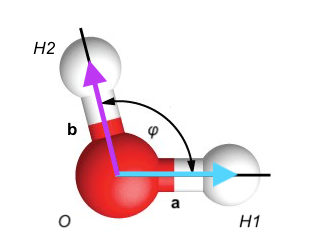
The bond length between H1 and O is given by the vector connecting these two atoms a in the image and can be computed using the above formula.

To determine the angle between two vectors you can use the scalar product:

\[\mathbf{a}\cdot \mathbf{b} = \vert\vert\mathbf{a}\vert\vert \,\vert\vert\mathbf{b}\vert\vert\cos \phi,\]

where $\mathbf{a}$ and $\mathbf{b}$ are vectors, and $\phi$ is the valence angle we are after. We need to solve the dot product according to the valence angle $\phi$ by rearranging the above equation:

\[\phi = \arccos\Big(\frac{\mathbf{a}\cdot\mathbf{b}}{\vert\vert\mathbf{a}\vert\vert \,\vert\vert\mathbf{b} \vert\vert}\Big)\]

You can use the math library to get the arccos of an angle, e.g.: math.acos()

The scalar product or dot product can be computed using np.dot() in Python.

def compute_angle_water(O_position,H1_position, H2_position):
    """This function computes the angle between two three atoms
    
    Parameters:
    -----------
    H1_position:numpy array 
        contains 3 entries as x, y and z coordinates
    O_position:numpy array
        contains 3 entries as x, y and z coordinates
    H2_position:numpy array
        contains 3 entries as x, y and z coordinates
    
    Returns:
    --------
    angle :float
        value of the angle
    """
    vector_of_bond_a = H1_position-O_position
    vector_of_bond_b = H2_position-O_position

    bond_length_a = compute_bond_length(H1_position, O_position)
    bond_length_b = compute_bond_length(O_position, H2_position)
    
    angle = m.acos(np.dot(vector_of_bond_a,vector_of_bond_b)/(bond_length_a*bond_length_b))
    return np.degrees(angle)
    

angle = compute_angle_water(position_atom_O,position_atom_H1,position_atom_H2)
print(f'The angle of a water molecule is: {angle:.2f}°.')

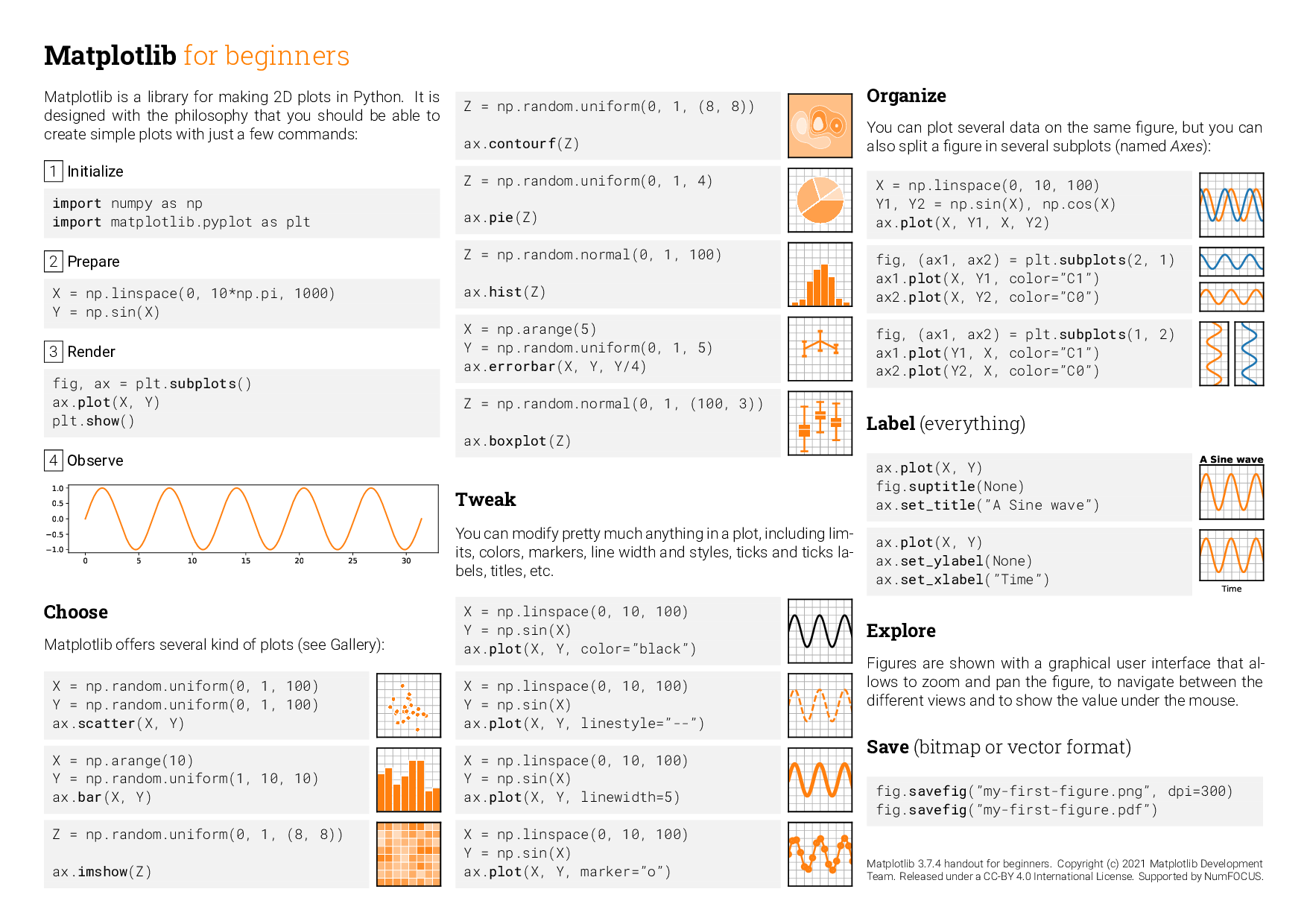
Recap: Reminder of further resources#

If you ever get stuck with Matplotlib, they have some very helpful cheatsheets, one of which is shown below:

Matplotlib beginner cheat sheet

1.2 Recap of plotting distributions #

Take a look at the following code:

# Generate 10000 random samples from a normal distriubution 
X = np.random.normal(4, 0.3, 10000)
# initiate the plot
fig, ax = plt.subplots()
fig.set_figwidth(4)
fig.set_figheight(4)
# Use numpy to compute a histogram
prob, edges = np.histogram(X, density = True, bins=30)
half_width = (edges[1]-edges[0])/2
bin_centres = edges[:-1]+half_width
# plot the probability density from the histogram
ax.plot(bin_centres, prob, marker="o", color="red")

How would you expect the final plot to look like?

Tasks 1 #

Task 1.1 : generate a 1D array, x, and plot x squared using non-default line types and colours, label the plot

Practice labelling your plot as well!

xlabel()
ylabel()
title()

Hint : To neatly write sub- and superscripts on the plots, like $x_2$ or $x^2$ in the example above, use the $LaTeX$ notation in the code - $x_2$ and $x^2$ respectively. For more examples see here.

# Task 1: Test out the solution in this cell:
# FIXME

Click here to see the solution to Task 1.1

# generating an array
x = np.linspace(-10, 10, 21) 
y = x**2

# plotting with x in a named colour, connected by a dotted line of a declared width
plt.plot(x, y, "x:", color="tomato", linewidth="1.5") 

# adding labeLs
plt.xlabel("x")
plt.ylabel("y")
plt.title("my plot $y=x^2$")

plt.show()

Task 1.2 : The file data/water.xyz contains a cluster of ice, i.e. many water molecules in a solid state. It has the xyz -file format and below is some help given how to read data from the file.

Take a look at how the file is read and make sure you understand it. This is one example way of reading this file. There are many other options too.
Compute the angle of each water molecule using the function defined above and append each angle to a list of angles.
Plot a distribution of from the list of angles and report its mean and standard deviation.

# Have a look at the data file first 
!head data/water.xyz

# reading the data in
# This generates a numpy array with the coordinates
data = np.genfromtxt('data/water.xyz', skip_header=1, usecols=[1,2,3])
# We don't want to use the first row and the first column this is what skup_header and use_cols does

# now we loop over this in threes to group the molecules together:
water_molecules = []
for i in range(0,len(data),3):
    # This selects each water molecule
    water_molecule = data[i:i+3]
    # Uncomment this line to see what is happening in detail
    # print(water_molecule)
    water_molecules.append(water_molecule)
print(f'We have {len(water_molecules)} water molecules in our file.')

# FIXME

Click here to see the solution to Task 1.2

# subtask 2
# computing angle
angles = []
for water in water_molecules:
    angle = compute_angle_water(water[0], water[1], water[2])
    angles.append(angle)
    
# subtask 3
# plotting the distribution
plt.hist(angles, bins=30)
plt.xlabel("angle in degree")
plt.ylabel("Count")

print(f"The mean is {np.mean(angles):.2f}")
print(f"The standard deviation is {np.std(angles):.2f}")

Task 1.3 : Working with data. Use the file data/anscombes_quartet.dat. This file is a tab delimiter file with 8 columns. The first and second columns make up one data set, the second and third the next one, and so forth.

Read the data into a pandas dataframe,
Create four subplots of the data,
Answer the mentimeter question.

# Task 3: Test out the solution in this cell:

# An example of naming the columns of the file
colnames=["X1", "Y1", "X2", "Y2", "X3", "Y3", "X4", "Y4"]

data = pd.read_csv(# FIXME
                   skiprows=2, names=colnames)

# Setup your 4 subplots
fig, axs = plt.subplots(2, 2)

# Set the figure size
fig.set_figwidth(8)
fig.set_figheight(8)

# add data to plot
axs[0, 0].scatter(data['X1'], data['Y1'])
# FIXME
# FIXME

# make sure it is labelled
for ax in axs.flat:
    ax.set(xlabel='x-data', ylabel='y-data')
    
for ax in axs.flat:
    ax.label_outer()

# Set the ranges of all axes
plt.setp(ax, xlim=(4,20), ylim=(3,13))

Click here to see the solution to Task 1.2

# Loading the dataset
colnames=["X1", "Y1", "X2", "Y2", "X3", "Y3", "X4", "Y4"]
data = pd.read_csv("data/anscombes_quartet.dat", delimiter="\t", skiprows=2, names=colnames)

# Setup your 4 subplots
fig, axs = plt.subplots(2, 2)
fig.set_figwidth(8)
fig.set_figheight(8)

# add data to plot
axs[0, 0].scatter(data["X1"], data["Y1"])
axs[0, 1].scatter(data["X2"], data["Y2"])
axs[1, 0].scatter(data["X3"], data["Y3"])
axs[1, 1].scatter(data["X4"], data["Y4"])

# make sure it is lablled
for ax in axs.flat:
    ax.set(xlabel="x-data", ylabel="y-data")
    
for ax in axs.flat:
    ax.label_outer()

# Setting the values for all axes.
plt.setp(ax, xlim=(4,20), ylim=(3,13))

Data is said to be perfectly correlated, if all points fall onto a straight line that is $x=y$. Take a look at your data: which of the four plots do you think is the most correlated?

Task 1.4 (advanced) : Working with data. Use the file data/ramachandran.dat. It contains dihedral angles of the backbone of a protein in two columns. Column 1 is the φ angle and column 2 the ψ angle. To find out more about Ramachandran diagrams take a look here, and for more on dihedral angles see here.

1. Read the data into a pandas dataframe,

2. Create a single plot that is a 2D density map of φ against ψ,

3. Make sure your plot is labelled correctly and displays a colour bar!

# Task 4: Test out the solution in this cell:

# 1. Read the data into a pandas dataframe, 
# FIXME
  
# 2. Create a single plot that is a 2D density map of $\phi$ against $\psi$
# FIXME

# 3. Make sure your plot is labelled correctly and displays a colour bar!   
# FIXME

Click here to see the solution to Task 1.4 (Advanced)

# Read in the dataframe
df = pd.read_csv("data/ramachandran.dat", 
                 skiprows=29, 
                 names=["phi", "psi"], 
                 usecols=[0,1], 
                 sep="\s+",
                 dtype=float)

# Check that we read it correctly
print(df.head())

# Get the columns
phi = df["phi"].to_numpy()
psi = df["psi"].to_numpy()

# Initialise figure object
fig, ax = plt.subplots(1,1)

# Plot a density plot as a 2D histogram
histogram, x_edges, y_edges, image = ax.hist2d(phi, psi, bins=(200, 200), cmap="RdYlGn_r", cmin=1)

# Add a colour bar
cbar = fig.colorbar(image, orientation="vertical")
cbar.set_label("Count")

# Add labels
ax.set_title("Ramachandran plot")
ax.set_xlabel("$\phi$")
ax.set_ylabel("$\psi$")

# Show plot
plt.show()

2. Computing Correlations#

Reminder: mean $\mu$ and standard deviation $\sigma$#

The mean $\mu$ is given by:

(6)#\[\begin{equation} \mu = \frac{1}{N} \sum_i^N x_i , \end{equation}\]

where $N$ is a number of samples, as as they increase the mean becomes closer to the ‘true’ value.

mu = np.sum(x) / len(x)

or with numpy: np.mean(x).

Note: Median is a middle value separating the greater and lesser halves of a data set, since the normal distribution is symmetric, mean and median are equivalent.

The standard deviation (STD), $\sigma$ quantifies how much the numbers in our set deviate from the mean, $\mu$

(7)#\[\begin{equation} \sigma = \sqrt{\frac{1}{N}\sum_{i=1}^N(x_i-\mu)^2}. \end{equation}\]

it can be written as:

sigma = np.sqrt( np.sum( ( x - np.mean(x))**2 ) / len(x) )

or with numpy np.std(x).

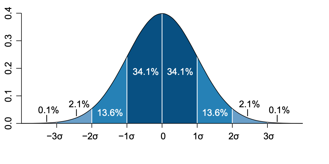
On a normal distribution the values that are less than 1 $\sigma$ away from the mean, $\mu$, will account for the 68.27% of the set - this is our confidence interval

2.1 Pearson’s correlation coefficient#

One way of quantifying the correlation between two datasets is to compute their Pearson’s correlation coefficient $R$.

If $R$ it is 1, or close to 1 the data is highly correlated,
around 0 the data is not correlated
when it is close to -1 the data is anticorrelated.

Mathematically the correlation coefficient is defined as:

$R = \frac{\langle(X-\mu_X)(Y-\mu_Y)\rangle}{\sigma_X\sigma_Y}$,

where $\sigma$ is the standard deviation of the data set $X$ or $Y$ and the symbol $\langle \cdot \rangle$ denotes computing the mean of the quantities inside the angular bracket.

The equation contains exactly what you learned last week!

Can you think of examples of correlated data?

Tasks 2 #

Task 2.1 : Write a function that computes the Pearson correlation coefficient between two datasets, making use of the numpy functions np.mean() and np.std() to compute the mean and standard deviation.

# Here is some data
number_generator = np.random.default_rng(12345)
X = 20 * number_generator.standard_normal(size=1000) + 100
Y = X + (10 * number_generator.standard_normal(1000) + 50)

# Task 1: Test out the solution in this cell:
def compute_pearson_r(X, Y):
    r''' function that computes the Pearson correlation coefficient
    Parameters
    ----------
    Computes the correlation between X and Y
    
    X : 1-d numpy array
        dataset 1
    Y : 1-d numpy array
        dataset 2
        
    Returns:
    --------
    R : float
        value of pearson R
    '''
    
    R = None
    
    # FIXME
    
    return R

Click here to see the solution to Task 2.1.

def compute_pearson_r(X,Y):
    r''' function that computes the Pearson correlation coefficient
    Parameters
    ----------
    Computes the correlation between X and Y
    
    X : 1-d numpy array
        dataset 1
    Y : 1-d numpy array
        dataset 2
        
    Returns:
    --------
    R : float
        value of pearson R
    '''
    
    R = None
    mean_x = np.mean(X)
    mean_y = np.mean(Y)
    std_x = np.std(X)
    std_y = np.std(Y)
    covariance = np.mean((X-mean_x)*(Y-mean_y))
    R = covariance/(std_x*std_y)
    
    return R

Task 2.2 : Does your function work correctly? Check if you get the same answers as from the built-in function pearsonr in the scipy.stats package.

from scipy.stats import pearsonr
# you use pearson r from the scipy.stats package in the following way:
# pearsonr(dataset1, dataset2)[0]

# Check what happens when you remove the [0] at the end and print the output. 

# Task 2: Test out the solution in this cell:
# FIXME

Click here to see the solution to Task 2.2

pearson1 = pearsonr(X, Y)[0]
pearson2 = compute_pearson_r(X, Y)
print(pearson1, pearson2)

Task 2.3 : Compute the correlation coefficient of all 4 datasets of the Anscombe's quartet. What do you observe?

# Task 3: Test out the solution in this cell:
# FIXME

Click here to see the solution to Task 2.3.

pearson1 = pearsonr(data["X1"], data["Y1"])[0]
pearson2 = pearsonr(data["X2"], data["Y2"])[0]
pearson3 = pearsonr(data["X3"], data["Y3"])[0]
pearson4 = pearsonr(data["X4"], data["Y4"])[0]
print(f"{pearson1}\n{pearson2}\n{pearson3}\n{pearson4}")

2.2. Spearman’s Rank Correlation Coefficient#

There are other ways of measuring correlation. Take a look at the documentation of the Spearman rank correlation coefficient in the scipy package here and a bit more background on it here.

Advanced Task 2.4 : Compute the Spearman's rank correlation coefficient for the Anscombe's quartet.

# Task 2.4: Test out the solution in this cell:
# FIXME

Click here to see solution to Task.

from scipy.stats import spearmanr
    
spearman1 = spearmanr(data["X1"], data["Y1"])[0]
spearman2 = spearmanr(data["X2"], data["Y2"])[0]
spearman3 = spearmanr(data["X3"], data["Y3"])[0]
spearman4 = spearmanr(data["X4"], data["Y4"])[0]
print(f"{spearman1}\n{spearman2}\n{spearman3}\n{spearman4}")

Break#

Next notebook#

Unit 07 Fitting II

Data-Driven Chemistry

Unit 07 Fitting Part I

Contents